Many of the common real-world problems have been well-defined and have efficient solvers. For example, the bin packing problem, Travelling Salesman Problem (TSP), shortest path in a graph etc, have been well-studied. Some other problems may be reduced to one of these NP-complete problems and any of the many off-the-shelf solvers can be used to solve them. Tremendous effort have been put into building efficient solvers and many of them are publicly available.
A curiosity may arise - to employ neural networks or any gradient-based learners with a combinatorial layer in their midst. For example, a simple path finding task may be given, but with unknown graph weights that must be inferred from the problem (say, a 2D image). This kind of obfuscations are far more common in real-world scenarios. In such cases, machine learning (gradient-based) models may be used to cast the problem suitable for the combinatorial solver.

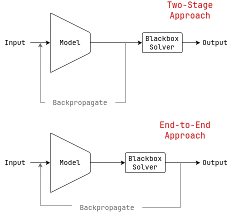
Two ways of combining gradient-based models with combinatorial solvers. Two-Stage (Top) and End-to-End (Bottom).
The two common ways to combine gradient-based models with combinatorial solvers are 1) two-stage, where the combinatorial solver is used as a post-processing step and the model is separately optimized via backpropagation and 2) end-to-end, where the combinatorial solver is part of the whole model and the whole model is optimized via backpropagation[1]. The two-stage approach is useful when the optimal costs / inputs to the solver is known. However, this limits its applicability as optimal costs are often unknown in real-world scenarios. The end-to-end approach is more applicable and will be the focus of this article.
Gradients Through Perturbation
Zeroth Order gradient estimation is a viable alternative for computing the gradients for non-differentiable functions or for those whose gradients are generally unavailable. In these techniques, the function to be differentiated is queried at multiple points and a finite-difference gradient estimator can be constructed.
Zeroth order optimization, however, may require large number of queries across various directions to get a good estimate of the gradient$-$for faster convergence[2]. Such directional gradients are required to get an unbiased estimator for the true gradient.
The standard way of computing the zeroth order gradient for a non-differentiable function $h(\vw)$ is as:
$$ \frac{dL}{d\vw} = \sum_{i}^{N} \frac{1}{\lambda} \left [h \left ( \vw + \lambda \vu_i \right) - h(\vw) \right ] \vu_i $$
Where $\vw$ is the input to the function $h$, $\vu$ is a random director vector, and $\lambda$ is a step-size/ smoothing factor / perturbation value as per the interpretation. Note that $N$ gets prohibitively high as the problem dimension increases. But we can greatly improve upon this based on the loss landscape of our end-to-end model.

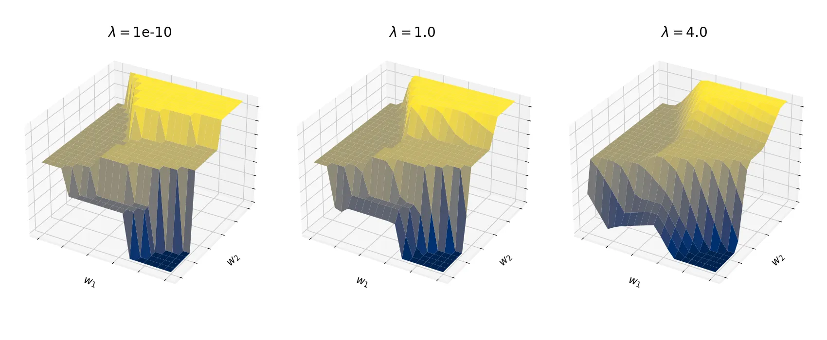
The Input-Output mapping for the Shortest-Path solver can be made piecewise affine by perturbation.
In the end-to-end approach, we have a model $f_{\theta}$ that predicts the inputs $\vw$ to the combinatorial solver $\texttt{BlackBoxSolver}$, which computes the final result $\vy$. The loss function $L$ is defined on the output of the solver $\vy$. During backpropagation, we get the gradient of the loss function $L$ with respect to the output of the solver $\vy=\texttt{BlackBoxSolver}(\vw)$ as $\nabla_{\vy}L$ and we require the gradient with respect to the input $\vw$ as $\nabla_{\vw}L$ to continue backpropagating through the model $f_{\theta}$.
The issue with combinatorial solvers is that the input-output relationship is piecewise constant. Although the gradient exists almost everywhere, it is a constant zero almost everywhere and undefined at the discontinuities. Refer to the figure above. It is thus, not sufficient to handle just the discontinuities, but also the piecewise constant nature of the solver.
Observe that the it is not necessary to relax the constraints of the solver to make it differentiable. The solver itself can be a blackbox and our concern is mainly the input-ouput ($\vw \to \vy$) mapping of the solver. Similar to equation (1), we can get gradient estimates without modifying the solver in any way. The trick is now to get informed directions $\vu$ along which we have to perturb the blackbox to get optimal (and sample-efficient) gradient estimates.
If we can convert the piecewise constant loss landscape to piecewise affine, then we can just take the gradients along the direction that has the maximum slope. During the backward pass, to perturb the predicted input $\hat{\vw}$ to the solver, we can use the gradient $\nabla_{\vy}L$ at the predicted output $\hat{\vy}$.
$$ \begin{aligned} \vw_\lambda &= \hat{\vw} + \lambda \nabla_{\vy} L(\hat{\vy}) \\ \vy_\lambda &= \texttt{BlackBoxSolver}(\vw_\lambda) \end{aligned} $$
Then the gradient is simply
$$ \nabla_w L(\hat{w}) = \frac{1}{\lambda} \left [y_\lambda - \hat{y}\right ] $$
For the case of shortest path, the solver could be $\texttt{Dijkstra}$ with $\vw$ being the edge weights, or for the knapsack problem or the scheduling problems, off-the-shelf solvers like Gurobi[3] can be used.
Although the above technique for combinatorial solvers was proposed in a 2020 ICLR paper [4], it is not novel. This kind of differentiation through perturbation was first proposed by Justin Domke in 2012[5], in a slightly different context. They show that
$$ \nabla_{\vw} L = \lim_{\lambda \to 0} \frac{1}{\lambda} \left [h \left ( \vw + \lambda \nabla_{h} L \right) - h(\vw)\right ] $$
Code
import torch
from typing import Tuple

def solver_func(inputs):
    """
    Combinatorial solver function.
    """
    ...


class BlackBoxSolver(torch.autograd.Function):
    @staticmethod
    def forward(ctx, weights: torch.Tensor, lambda_val:float):
        """
        Forward pass of the combinatorial solver layer.

        Args:
            ctx: context for backpropagation
            weights (torch.Tensor): input for the solver
            lambda_val: perturbation parameter

        Returns:
            Result of the solver.
        """
        device = pred_costs.device
        pred_costs = pred_costs.detach().cpu().numpy()
        ctx.lambda_val = lambda_val
        solver_result = np.asarray([solver_func(arg) for arg in list(pred_costs)])

        ctx.save_for_backward(pred_costs, solver_result)
        return torch.from_numpy(solver_result).float().to(device)

    @staticmethod
    def backward(ctx, grad_output: torch.Tensor) -> Tuple:

        pred_costs, solver_result = ctx.saved_tensors
        assert grad_output.shape == solver_result.shape

        # Get the gradient output of the previous layer
        grad_output_numpy = grad_output.detach().cpu().numpy()

        # Get perturbed costs as input for the combinatorial solver
        pert_costs = np.maximum(pred_costs + ctx.lambda_val * grad_output_numpy, 0.0)

        # Pass the perturbed weights through the solver to get corresponding results
        solver_result_pert = np.asarray([solver_func(arg) for arg in  list(pert_costs)])

        # Compute the gradient estimate
        gradient = -(solver_result - solver_result_pert) / ctx.lambda_val
        return torch.from_numpy(gradient).to(grad_output.device), None
The downside of the above technique is that the smoothed loss landscape can be come non-convex, even if the original loss was convex. The earlier figure shows that as $\lambda$ increases, the loss landscape becomes dramatically different, where some optima are even lost. In fact, $\lambda$ must be high enough to make the landscape piecewise affine. This actually goes against the idea of step sizes being small ($\lambda \to 0$) in usual finite-difference methods (refer the limit in equation (4)).
The perturbation value $\lambda$ is, therefore, quite important while training - where a balance between the smoothness of the loss landscape and the optimality of the solution must be struck. The general rule of thumb is to make sure that the magnitude of $\vw_\lambda$ is not heavily altered from $\vw$.
| [1] | For a quick overview of some general techniques for such problems, refer to the following: Tang, Bo, and Elias B. Khalil. Pyepo: A pytorch-based end-to-end predict-then-optimize library for linear and integer programming. Mathematical Programming Computation 16.3 (2024): 297-335. ArXiv Link. |
| [2] | Berahas, Albert S., et al. A theoretical and empirical comparison of gradient approximations in derivative-free optimization. Foundations of Computational Mathematics 22.2 (2022): 507-560. ArXiv Link. |
| [3] | LLC Gurobi Optimization. Gurobi optimizer reference manual, 2019. URL: http://www.gurobi.com |
| [4] | Pogančić, Marin Vlastelica, et al. Differentiation of blackbox combinatorial solvers. International Conference on Learning Representations. 2020. |
| [5] | Domke, Justin. Implicit differentiation by perturbation. Advances in Neural Information Processing Systems 23 (2010). PDF Link |