Fourier Neural Operators (FNOs)[1] have been quite successful to say the least with a variety of immediate practical applications from accurate high-resolution weather forecasting, Carbon Capture and Storage (CCS) simulations, industrial-scale automotive aerodynamics, and material deformation to name a few[2].
Here's a quick overview of FNOs $-$ Recall that the general form for a Neural Operator as a composition of layers $v$ of the form[3]
$$ v^{l+1}(\vx) := \sigma \left (\vW v^l(\vx)+ \int_\fX k(\vx,\vz) v^l (\vz) d \vz \right ) $$
Where $\sigma$ is the usual pointwise nonlinearity, and $k$ is some kernel function. The motivation here is that, to learn an operator as a mapping between functions, we have to go beyond just pointwise transformations like $\vW v(\vx)$. The integral part in the above equation defines a family of functional transforms called Kernel Integral Transformations, thus enabling the network to learn a more general form of the input-output functional mapping. The integral over the input domain $\fX \subset \R^d$ ensures that the network is not restricted to learning the fixed number of input function measurements or their locations.
We can identify that the integral term represents a convolution operation, provided the kernel $k$ is stationary (translation invariant) i.e $k(\vx, \vz) = k(\vx - \vz)$. This immediately suggests the use of Fourier transforms to convert the convolution to matrix multiplication, which is computationally more efficient than computing the integral directly.
$$ \int_\fX k(\vx, \vz) v(\vz) dz = \int_\fX k(\vx-\vz) v(\vz) dz = \fF^{-1}(\fF(k) \cdot \fF(v))(\vx) $$
Therefore, instead of designing a network to learn the kernel $k: \fX \to \R^{d_v \x d_v}$, we now directly learn its Fourier transform $\fF(k)$, represented as $R_{\phi}$.
$$ v^{l+1} (\vx) := \sigma \left (\vW v^l(\vx)+ \fF^{-1}(R_{\phi} \cdot \fF(v^l))(\vx)\right ) $$
Here, I would like to point out that the above equation has the form of a residual layer (you may have to squint hard). I find it funny that DNN researchers have this obsession about showing that their layer architecture looks like a residual layer. Anyhow.
Here, we note a couple of things $-$ FNOs work on uniformly discretized domains $\fX$; and the kernel $k$ is assumed to be periodic and bandlimited.
- A uniformly discrete domain implies that we can use FFT and IFFT.
- A periodic kernel means that we can parameterize $R_\phi$ in terms of discrete Fourier modes $p$, and a bandlimited kernel means that we can truncate the Fourier series to some maximum value $p_{\text{max}}$, resulting in a finite-dimensional representation of $R_\phi$ - a complex-valued tensor of size $(p_{\text{max}} \x d_v \x d_v)$[4].
These assumptions (a total of 3 including the stationary assumption) are crucial for an efficient practical implementation of FNOs. In the actual implementation of FNOs, there is a neat little trick[5] for computing this Fourier multiplication. Refer to a typical implementation for 2D inputs shown below - $R$ is no where to be seen! and what are those weights1 and weights2?
# Reference: https://github.com/neuraloperator/neuraloperator/blob/13c7f112549bfcafe09a4c5512a90206141b3511/neuralop/layers/spectral_convolution.py#L526

import torch
import torch.nn as nn

class FourierLayer2D(nn.Module):
    def __init__(self,
                 d_in: int,
                 d_out: int,
                 modes1: int,
                 modes2: int):
        """

        Fourier Layer for 2D inputs. Computes the following operation:

        v_{l+1} = F^{-1}( F(v_l) * R )

        where F is the Fourier Transform, R is the kernel's Fourier coefficients,

        Args:
            d_in: int: Dimension of input
            d_out: int: Dimension of output
            modes1: int: Max number of modes in the x-direction
            modes2: int: Max number of modes in the y-direction

        """
        super(FourierLayer2D, self).__init__()

        self.d_in   = d_in
        self.d_out  = d_out
        self.modes1 = modes1
        self.modes2 = modes2

        self.scale = (1 / (d_in * d_out))

        # Set the complex weights to parameterize the
        # Kernel's Fourier coefficients R.
        self.weights1 = nn.Parameter(self.scale *
                                    torch.rand(d_in,
                                               d_out,
                                               self.modes1,
                                               self.modes2, dtype=torch.cfloat))
        self.weights2 = nn.Parameter(self.scale *
                                     torch.rand(d_in,
                                                d_out,
                                                self.modes1,
                                                self.modes2, dtype=torch.cfloat))

    def forward(self, v: torch.Tensor):
        batchsize, M, N = v.shape[0], v.shape[-2], v.shape[-1]

        # Compute Fourier transform of the
        # input tensor v. Note that this is the
        # output of the previous layer.
        v_ft = torch.fft.rfft2(v)

        # Truncate the Fourier modes and multiply with the
        # weight matrices
        out_ft = torch.zeros(batchsize,
                             self.d_out,
                             M,
                             N//2 + 1,
                             dtype=torch.cfloat, device=v.device)

        out_ft[:, :, :self.modes1, :self.modes2] = \
            self.compl_mul2d(v_ft[:, :, :self.modes1, :self.modes2], self.weights1)
        out_ft[:, :, -self.modes1:, :self.modes2] = \
            self.compl_mul2d(v_ft[:, :, -self.modes1:, :self.modes2], self.weights2)

        # Inverse Fourier Transform to get the layer outputs in
        # the input physical space.
        v = torch.fft.irfft2(out_ft, s=(v.size(-2), v.size(-1)))
        return v

    def compl_mul2d(self, tensor1: torch.Tensor, tensor2: torch.Tensor):
        # (batch, d_in, x,y ), (d_in, d_out, x,y) -> (batch, d_out, x,y)
        return torch.einsum("bixy,ioxy->boxy", tensor1, tensor2)
Let's try to understand what's happening here. The 2D output tensor $\vv \in \R^{d_v \x M \x N}$ of the previous layer is the input to the current layer and is Fourier transformed using rfft2. Since the input is real-valued, the corresponding Fourier transform is Hermitian and therefore, it is efficient to use rfft2 instead of fft2. Therefore, $\fF(\vv) \in \C^{d_v \x M \x (N/2 + 1)}$ and correspondingly the result of the spectral operation (equation (2)) $\in \C^{d_v \x M \x (N /2 + 1)}$ (note fewer parameters).
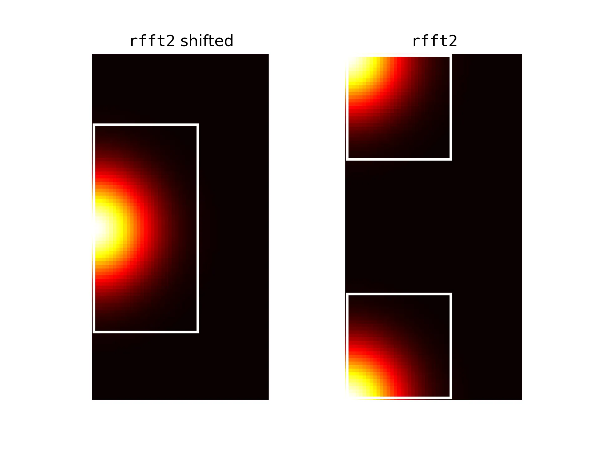
Truncating Fourier modes using rfft2. The white boxes show the boundary for truncation. (right) The top half represents positive modes, while the bottom half represent negative modes.
Now, the trick is in understanding that during truncation, we have to consider both the positive and negative Fourier modes. Our actual range of truncation is $[-p_{\text{max}}, p_{\text{max}}]$ . If the input domain is discretized into $N$ and $M$ points along respective dimensions, we truncate the Fourier modes as v_ft[:, :, :self.modes1, :self.modes2] (positive frequencies) and v_ft[:, :, -self.modes1:, :self.modes2] (negative modes). This can be verified based on the figure above. Therefore, in practice, instead of one $R$ matrix, we decompose it into two $R_1, R_2 \in \C^{p_{\text{max}} \x q_{\text{max}} \x d_v \x d_v}$ matrices, each corresponding to the positive and negative Fourier modes respectively. This results in a more efficient implementation that is extensible to higher dimensions as well[6].
| [1] | Li, Z., Kovachki, N., Azizzadenesheli, K., Liu, B., Bhattacharya, K., Stuart, A., & Anandkumar, A. (2020). Fourier neural operator for parametric partial differential equations. arXiv preprint arXiv:2010.08895. |
| [2] | For a more detailed presentation of the applications of Neural Operators in general, refer to - Azizzadenesheli, K., Kovachki, N., Li, Z., Liu-Schiaffini, M., Kossaifi, J., & Anandkumar, A. (2024). Neural operators for accelerating scientific simulations and design. Nature Reviews Physics, 1-9. |
| [3] | The general form was described in the paper - Li, Zongyi, et al. Neural operator: Graph kernel network for partial differential equations. arXiv preprint arXiv:2003.03485 (2020). |
| [4] | The bandlimited assumption may not always hold and yet we truncate to $p_{\text{max}}$ modes. Hence, it is usualy recommended to play around with the maximum frequency $p_{\text{max}}$ for each application. The original FNO paper recommends $p_{\text{max}, j} = 12$ for each channel/feature dimension $j$. |
| [5] | A clean implementation of the Fourier multiplication can be found here. |
| [6] | This trick was actually explained in the paper - Kossaifi, J., Kovachki, N., Azizzadenesheli, K., & Anandkumar, A. (2023). Multi-grid tensorized Fourier neural operator for high-resolution PDEs. arXiv preprint arXiv:2310.00120. |