The $l_1$ regularized optimization problems are quite common in machine learning. They lead to a sparse solution to the modelling problem. Consider the following optimization problem with $l_1$ penalty[1].
$$ \min_{\theta \in \R} f(\theta) := h(\theta) + \lambda |\theta| $$
Where $\theta$ are the parameters of the model $f$ to be optimized. Let us study the reparameterization $\theta = \mu \circ \nu$ for all $\theta \in \R$, where $\circ$ represents the element-wise (Hadamard) product of the vectors $\mu$ and $\nu$. This is called the Hadamard product parameterization (HPP) or simply the Hadamard paramterization[2]. Then the equation (1) can be written as
$$ \begin{aligned} \min_{\theta \in \R} f(\theta) &= h(\theta) + \lambda |\theta| \\ &\leq h(\theta) + \lambda \|\theta\|_2 \\ &=h(\mu \circ \nu) + \lambda \sum_i |\mu_i \nu_i| \\ &= h(\mu \circ \nu) + \lambda \sum_i \sqrt{\mu_i^2 \nu_i^2} \\ &\leq h(\mu \circ \nu) + \lambda \bigg ( \sum_i \frac{\mu_i^2 + \nu_i^2}{2} \bigg ) && {\color{OrangeRed}\text{AM-GM Inequality}}\\ &\leq h(\mu \circ \nu) + \frac{\lambda}{2} \big ( \| \mu\|_2^2 + \|\nu\|_2^2 \big ) \\ & \leq \min_{\mu, \nu \in \R} g(\mu, \nu) \end{aligned} $$
Therefore, the auxiliary optimization function is $$ \min_{\mu, \nu \in \R} g(\mu, \nu) := h(\mu \circ \nu) + \frac{\lambda}{2} \big ( \| \mu\|_2^2 + \|\nu\|_2^2 \big ) $$
The above function is constructed rather purposefully to satisfy the following properties.
- The over-parameterized function $g(\mu, \nu)$ is an upper bound to our optimization function $f(\theta)$, i.e. $g(\mu,\nu) \geq f(\mu \circ \nu), \forall \mu,\nu \in \R$. The equality occurs where $|\mu| = |\nu|$ as can be observed from equation (2).
- The function $g(\mu, \nu)$ satisfies the equality $\inf f = \inf g$. This means that the optima (minima in this case) of $f$ is equal to the optima of $g$. In other words, if $\mu$ and $\nu$ are optimal (in terms of $l_2$), then $\mu \circ \nu$ is an optimal (in terms of $l_1$) value of $\theta$.
Moreover, since $g(\mu, \nu)$ uses the $l_2$ regularization, it is differentiable and biconvex. Thus, the auxiliary function is amenable to gradient-based optimization algorithms like SGD, Adam, etc. Interestingly, Ziyin et. al.[3] also proved a stronger property compared to $\inf f = \inf g$. They show that at all stationary points of (3), $|\mu_i| = |\nu_i| \; \forall i $ and every local minima of $g(\mu, \nu)$, given by equation (3) is a local minima of $f(x)$, given by equation (1).
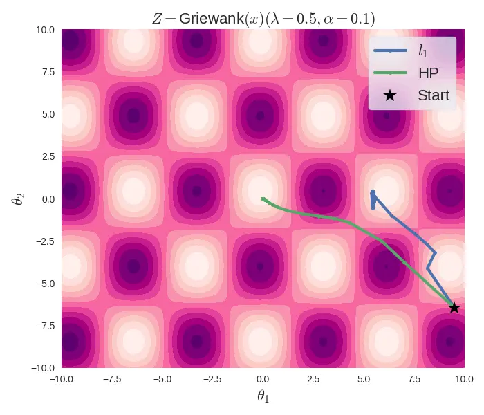
Optimization trajectory of l1 and HP regularizations
The above figure shows that, for the same initial conditions and optimization parameters, the $l_1$ regularized objective function (Griewank, in this case) gets stuck in a local minima, while the Hadamard-parameterized function correctly reaches the global minima, which is at $(0, 0)$. Note that the $l_1$ regularized objective can be used with Pytorch's SGD optimizer, as they use a subgradient of 1 at the non-differentiable point. But this is a convention, as the subgradient of $|x|$ at $0$ is the set $[-1, 1]$.
Lastly, similar to interpreting the $l_1$ and $l_2$ regularizers in least-squares problems as Laplacian and Gaussian priors respectively, the equation (3) can also be examined through a probabilistic framework. Here, with the parameters $\mu$ and $\nu$ subject to $l_2$ norm regularization, they can be construed as being governed by a Gaussian prior distribution $\mathcal{N}(0, 2/\lambda)$. This implies a regularization effect on the components $\mu$ and $\nu$.
| [1] | TIL, that the notation $l_p$ is reserved for vectors while the uppercase notation $L_p$ is for operators and functions. So, the appropriate notations are $l_2(x)$ and $L_2[\phi(x)]$ for vector $x$ and the function $\phi(x)$ respectively. |
| [2] | Hoff, P. D. (2017). Lasso, fractional norm and structured sparse estimation using a hadamard product parametrization. Comput. Stat. Data An., 115:186–198. ArXiv Link. |
| [3] | Ziyin, L. & Wang, Z. (2023). spred: Solving L1 Penalty with SGD. Proceedings of the 40th International Conference on Machine Learning, in Proceedings of Machine Learning Research 202:43407-43422 ArXiv Link |